Introduction
In modern pharmaceutical development and quality control, dissolution testing is more than a compendial requirement; it is a critical bridge between a drug’s formulation design and its clinical performance. By studying how a solid oral dosage form releases its active ingredient into solution, scientists can predict in vivo behavior, ensure batch-to-batch consistency, and meet regulatory expectations for safety and efficacy.
READ the whole dissolution test series
One of the most widely accepted tools for comparing dissolution profiles is the similarity factor (f₂). Regulatory agencies, such as the FDA, EMA, WHO, and USP, recommend f₂ as the statistical standard for demonstrating that two drug products, whether generic versus innovator or pre-versus post-change batches, behave equivalently in vitro. The correct interpretation of dissolution data and the accurate calculation of f₂ are therefore essential for bioequivalence assessments, method development, and global regulatory submissions.
This article provides a step-by-step guide to help pharmaceutical scientists, QC analysts, and regulatory professionals:
- Generate and interpret dissolution profiles with scientific accuracy.
- Apply the similarity factor (f₂) correctly to establish equivalence.
- Identify and resolve common pitfalls that can compromise results.
- Align laboratory practices with international guidelines to ensure acceptance.
By the end of this guide, you will not only understand the mathematical calculation of f₂, but also gain the ability to interpret dissolution profiles in context, defend your data during audits, and confidently prepare regulatory submissions.
Step 1: Collect High-Quality Dissolution Data
Before interpretation or statistical comparison can begin, the foundation of a reliable analysis lies in generating robust and reproducible dissolution data. Poorly designed or inconsistently executed tests will compromise every subsequent step, including calculation of the similarity factor (f₂).
1.1 Validate Your Method First
A dissolution profile is only as good as the method that produced it. International guidelines, including USP <711> Dissolution and the FDA Dissolution Testing Guidance, stress that the test method must be scientifically justified and validated. This includes:
- Apparatus Selection: Choose the appropriate USP apparatus (Paddle – Apparatus 2, Basket – Apparatus 1, Flow-through – Apparatus 4) based on dosage form. For immediate-release tablets, paddles (Apparatus 2) are the most common.
- Medium Selection: Use physiologically relevant pH conditions (1.2, 4.5, 6.8) unless a justified surfactant or special medium is needed to achieve sink conditions.
- Agitation Speed & Volume: Typically 50–75 rpm and 500–900 mL, chosen to balance discriminatory power with clinical relevance.
- Temperature Control: Maintain 37 ± 0.5 °C throughout the test to mimic body conditions.
1.2 Sampling Plan & Time Points
For an f₂ comparison to be valid, 12 dosage units per product must be tested, and at least three or more time points should fall within the 20–80% dissolution range. General best practices include:
- Early time point (to detect burst release or lag phase).
- Middle time point (around 50% release, informative for f₂).
- Late time point (where dissolution approaches plateau, usually ≥ 85%).
- Sampling intervals must be consistent (e.g., 5, 10, 15, 30, 45, 60 min for IR tablets).
1.3 Analytical Assay Accuracy
Whether using UV spectrophotometry or HPLC, analysts must ensure:
- Specificity: No interference from excipients or degradation products.
- Filter Compatibility: Filters should not adsorb analyte or release particles.
- Solution Stability: Confirm the drug remains stable in the medium for the test duration.
1.4 Reducing Variability
High variability in unit-to-unit dissolution curves can invalidate an f₂ calculation. To minimize this risk:
- Verify dosage form uniformity (content and hardness).
- Ensure proper deaeration of media (e.g., vacuum filtration or sonication).
- Calibrate the apparatus regularly to avoid misalignment or wobble.
Step 2: Plot and Visualize the Dissolution Profiles
Once high-quality data has been collected, the next step is to convert raw numbers into interpretable visuals. Dissolution data are inherently time-dependent, and plotting the results allows analysts to quickly detect patterns, anomalies, or inconsistencies before moving to statistical comparison.
2.1 Create a Dissolution Profile Graph
A standard dissolution profile is a line graph of % drug dissolved vs. time, with one curve for each unit or the mean profile (with error bars).
Best practices for plotting:
- X-axis: Time (minutes or hours).
- Y-axis: % drug dissolved.
- Overlay test and reference product curves.
- Include mean ± standard deviation for clarity.
- Use consistent scaling across batches for easy comparison.
Tip
Graphing software such as Microsoft Excel, GraphPad Prism, or DDSolver (Excel add-in) is commonly used in the industry.
2.2 Interpret Key Time Points
Beyond the full curve, certain summary parameters provide quick insight:
- t10% (lag time): Indicates the onset of dissolution. Longer lag may reflect slower disintegration.
- t50% (half-life of release): Highlights the mid-point of drug release.
- t80% (approach to plateau): Shows how quickly the dosage form reaches near-complete release.
Tip
These metrics allow qualitative comparison before applying mathematical tests. For instance, if the test product consistently lags behind the reference in reaching 50% release, an f₂ ≥ 50 may still be difficult to achieve.
2.3 Look for Visual Similarity and Red Flags
While the f₂ factor provides statistical confirmation, regulators still expect analysts to demonstrate visual similarity:
- Curves should follow the same trajectory without major crossings.
- The slope of dissolution should be comparable.
- Plateaus should occur within a similar range.
Red flags include:
- Large variability between units.
- Incomplete release (< 85% dissolved).
- Profiles that diverge significantly at early or middle time points.
2.4 Why Visualization Matters
Regulatory guidelines (FDA, EMA, WHO) emphasize that dissolution profiles should be both statistically and visually comparable. Even if an f₂ calculation gives a borderline result, a strong visual match strengthens your justification during regulatory submission.
Step 3: Qualitative Comparison of Dissolution Profiles
Before diving into numerical calculations like the similarity factor (f₂), regulators encourage a qualitative comparison of the dissolution curves. This step is about building a visual and scientific narrative: do the test (T) and reference (R) products behave in the same way when exposed to identical conditions?
3.1 Overlay the Test and Reference Profile
The first action is to overlay the T and R curves on a single graph. This allows a quick side-by-side comparison:
- Are both curves rising at the same rate?
- Do they reach a plateau at similar times?
- Is the final extent of drug release comparable?
Tip
Always use the same scale and axis labels when plotting multiple profiles. Misaligned scales can give a misleading impression of similarity.
3.2 Assess the Shape of the Curves
The shape of the dissolution curve reflects the underlying drug release mechanism. Analysts should qualitatively check:
- Initial phase: Is the lag time comparable? If one curve shows delayed release, it may indicate differences in disintegration or coating.
- Middle phase: Do the slopes (release rates) look parallel? Diverging slopes often suggest formulation differences.
- Terminal phase: Do both reach the same plateau (% release)? If one levels off significantly below 85%, it may fail regulatory expectations.
3.3 Variability Across Units
Dissolution is tested on six or more units. Visual comparison should also consider variability between units:
- Are the curves tightly clustered, or do some units deviate significantly?
- Does the test product show higher variability than the reference?
3.4 Apply Basic Acceptance Heuristics
Some quick rules of thumb are often used before statistical testing:
- If ≥ 85% drug release occurs within 15 minutes for both T and R, many agencies accept the products as similar without f₂ calculation (known as the “rapidly dissolving” exemption).
- If both curves show parallel trajectories with only minor shifts, statistical confirmation via f₂ is more likely to succeed.
- If curves cross each other or show inconsistent slopes, regulators may question the equivalence even if f₂ ≥ 50.
3.5 Regulatory Expectation on Qualitative Checks
According to FDA, EMA, and WHO guidelines, f₂ should not be interpreted in isolation. Agencies explicitly require visual inspection of profiles as a complementary step.
Step 4 : Statistical Assessment Using the Similarity Factor (f₂)
Once the dissolution curves have been visually compared, the next step is to provide quantitative confirmation of similarity. The most widely accepted statistical tool is the similarity factor (f₂), recommended by the FDA, EMA, WHO, and USP.
The f₂ test transforms the differences between the test (T) and reference (R) dissolution profiles into a single score ranging from 0 to 100. A higher value indicates greater similarity.
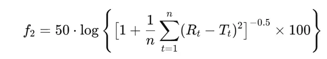
4.1 The f₂ Equation
The similarity factor is defined as:

Where:
- n = number of sampling time points (excluding 0 min)
- Rₜ = % drug dissolved from reference at time t
- Tₜ = % drug dissolved from the test at time t
4.2 Acceptance Criteria
Regulatory agencies generally apply the following thresholds:
- f₂ ≥ 50 → Profiles are considered similar (average difference ≤ 10% at each time point).
- f₂ < 50 → Profiles are considered dissimilar.
Tip
An f₂ value of 50 corresponds to an average difference of ~10% between profiles.
4.3 Conditions for f₂ Calculation
To ensure valid results, specific conditions must be met (FDA, EMA, WHO):
- Number of Units: At least 12 dosage units per product (test and reference).
- Time Points: Use 3 to 4 sampling points in the profile, excluding 0 min, and avoid the final point if both products release > 85%.
- Variability Constraint: The coefficient of variation (CV) should be ≤ 20% at the first time point and ≤ 10% at later points.
- No Mean Correction: Use untransformed mean values; do not normalize or smooth curves.
- Same Conditions: Dissolution media, RPM, and temperature must be identical.
4.4 Interpreting Results in Context
While f₂ ≥ 50 is a clear statistical signal, regulators emphasize that this result must be interpreted together with qualitative inspection:
- Consistent + f₂ ≥ 50 → Strong evidence of similarity.
- Crossing curves, but f₂ ≥ 50 → Regulators may still request additional justification.
- f₂ < 50 but visually close curves → May allow alternative statistical modeling (e.g., bootstrap, model-dependent approaches).
4.5 Common Pitfalls and Best Practices
- ❌ Using too many time points: Including unnecessary late-stage points where both profiles plateau can artificially inflate f₂.
- ❌ Ignoring variability: High unit-to-unit variability can mask true differences.
- ✅ Pre-define time points during method validation, don’t select points after data collection.
- ✅ Report full data: Include both the f₂ value and the raw profiles in regulatory submissions.
4.6 Regulatory Guidance
- FDA (2018): “An f₂ value of 50 or greater suggests sameness of the two profiles; however, graphical comparison should always complement statistical results.”
- EMA (2010): “The similarity factor should be calculated using the mean data of 12 units. Conditions for calculation must be strictly followed.”
- WHO (2006): “If more than 85% drug is dissolved within 15 minutes for both products, profiles can be considered similar without f₂ calculation.”
Step 5: Handling Cases Where f₂ Cannot Be Applied (Alternative Approaches)
While the similarity factor (f₂) is the gold standard for comparing dissolution profiles, there are scenarios where its application is not valid or not recommended. In such cases, alternative statistical and model-based approaches are required to ensure scientific and regulatory acceptance.
5.1 When f₂ Cannot Be Applied
You should avoid using f₂ in the following situations (FDA, EMA, WHO):
- High Variability in Results
- CV > 20% at early time points or > 10% at later points.
- Common with poorly soluble drugs (BCS Class II/IV).
- Too Few Sampling Points
- If dissolution completes too quickly (< 85% release within 15 minutes), f₂ is unnecessary (profiles are automatically similar).
- Too Many Sampling Points
- Including irrelevant late-stage plateau points artificially inflates f₂.
- Modified-Release Dosage Forms
- f₂ is validated primarily for immediate-release (IR) formulations. Extended-release (ER) products often require model-dependent analysis.
5.2 Alternative Approaches
- A. Multivariate Statistical Methods
- Mahalanobis distance or Hotelling’s T² test can evaluate differences across multiple time points simultaneously.
- Useful when variability is high but profiles still appear visually comparable.
- B. Model-Dependent Methods
- Fit dissolution data to mathematical models:
- Zero-order, First-order, Higuchi, Hixson–Crowell, Weibull.
- Compare model parameters between test and reference products.
- EMA and WHO recommend Weibull modeling for modified-release formulations.
- Fit dissolution data to mathematical models:
- C. Bootstrap f₂ Method
- Instead of a single mean-based calculation, generate confidence intervals for f₂ using resampling (e.g., 1,000 bootstraps).
- Acceptable if the lower bound of the 90% CI ≥ 50.
- FDA recognizes bootstrap as an advanced tool for highly variable data.
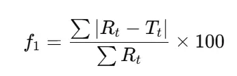
- D. f₁ Difference Factor
- Although less discriminative, the difference factor (f₁) may be used in conjunction with f₂:
- f₁ values ≤ 15 generally indicate similarity.
- Rarely used alone, but may supplement borderline f₂ cases.
5.3 Best Practices in Reporting Alternatives
- Always justify why f₂ was not applicable (e.g., high variability, MR formulation).
- Provide both graphical and statistical evidence.
- Clearly state the method used, assumptions, and results.
- Include regulatory references in the submission to strengthen credibility.
5.4 Regulatory Guidance
- FDA (2018): Acknowledges bootstrap methods and multivariate approaches when standard f₂ is invalid.
- EMA (2010): Encourages model-dependent analysis for MR formulations.
- WHO (2006): Recommends Weibull modeling for global harmonization of ER/MR comparisons.
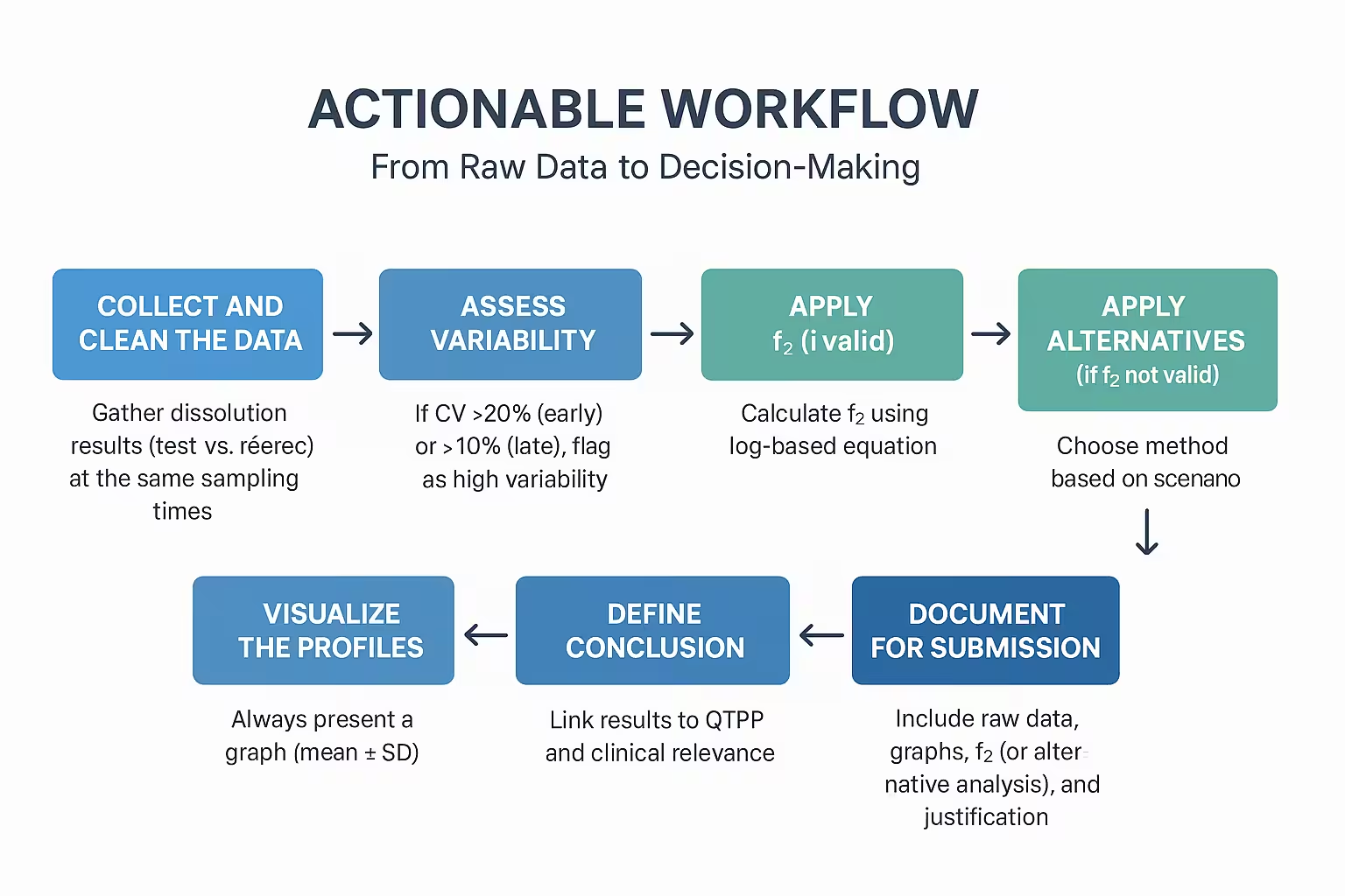
Step 6:Actionable Workflow: From Raw Data to Decision-Making
This step provides a practical framework for moving from dissolution test results → similarity evaluation → regulatory decision-making. Think of it as your playbook whenever you compare profiles.
6.1 Step-by-Step Workflow
Step 1: Collect and Clean the Data
- Gather dissolution results (test vs reference) at the same sampling times.
- Exclude points after 85% dissolution.
- Ensure ≥ 3 replicates per product.
- Calculate the mean % dissolved and %RSD.
Step 2: Assess Variability
- If %CV > 20% (early) or > 10% (late), flag as high variability.
- Consider bootstrap or model-dependent approaches.
Step 3: Apply f₂ (if valid)
- Calculate f₂ using the log-based equation.
- Decision rule: f₂ ≥ 50 → profiles similar.
- Document mean, SD, and final value.
Step 4: Apply Alternatives (if f₂ not valid)
- Choose a method based on the scenario:
- Bootstrap f₂ → high variability.
- Weibull/modeling → MR formulations.
- Multivariate stats → multiple-variable assessment.
Step 5: Visualize the Profiles
- Always present a graph (mean ± SD).
- Overlay test and reference profiles.
- Label axes clearly (% dissolved vs time).
Step 6: Define Conclusion
- Link results to QTPP and clinical relevance.
- State whether the product is:
- Comparable (suitable for biowaiver or regulatory submission).
- Non-comparable (further investigation required).
Step 7: Document for Submission
- Include raw data, graphs, f₂ (or alternative analysis), and justification.
- Reference FDA/EMA/WHO guidelines.
- Keep analysis reproducible (share spreadsheets/scripts if possible).
6.2 Example Decision Flow
Data Cleaned & Valid?
- ✅ Yes → Proceed to variability check.
- ❌ No → Re-run or correct experimental issues.
Variability Acceptable?
- ✅ Yes → Apply f₂.
- ❌ No → Apply bootstrap/modeling.
f₂ ≥ 50 or Alternative Confirms Similarity?
- ✅ Yes → Conclude profiles are similar.
- ❌ No → Profiles not comparable; investigate formulation/process issues.
6.3 Practical Notes for Analysts
- Always run at least 12 units when bioequivalence is intended.
- Keep records of medium prep, deaeration, and apparatus calibration.
- For MR products, report multi-time point acceptance criteria.
- Highlight both numerical and visual evidence in reports.
Step 7: Apply Statistical Tools for Profile Comparison
Once you have generated and plotted the dissolution profiles, the next critical step is statistical comparison. This ensures that any observed differences between the test and reference product are not just due to random variation but are scientifically and statistically meaningful.
Here’s how to apply statistical tools step by step:
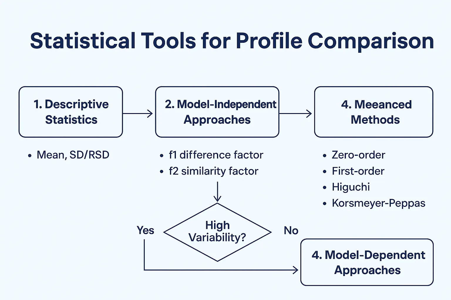
1. Begin with Descriptive Statistics
Before diving into advanced models, summarize your data using descriptive measures:
- Mean dissolution values at each time point
- Standard deviation (SD) or % Relative Standard Deviation (%RSD)
- Coefficient of variation (CV) to assess consistency
This provides a quick overview of data spread and variability across units.
2. Use Model-Independent Approaches (Similarity/Dissimilarity Factors)
The f1 (difference factor) and f2 (similarity factor) are the most widely accepted tools for comparing dissolution profiles:
- f1 (difference factor): Measures the relative error between two profiles.
- Formula:

- Acceptance: 0–15 indicates minor difference.
- f2 (similarity factor): Measures the closeness between two curves.
- Formula:
- Acceptance: 50–100 indicates similarity.
Note
Regulators like the FDA, EMA, and WHO recognize f2 ≥ 50 as a valid indicator of profile similarity for immediate-release (IR) products.
3. Consider Variability Adjustments
If your product shows high variability, the simple f2 approach may not be sufficient. In such cases, agencies recommend:
- Bootstrap methods (resampling-based confidence intervals for f2)
- Multivariate statistical distance (MSD) models
- Dissolution efficiency (DE%) comparisons
4. Apply Model-Dependent Approaches (Kinetic Models)
For a deeper mechanistic understanding, dissolution data can be fitted into mathematical models such as:
- Zero-order model (constant release rate)
- First-order model (release proportional to drug remaining)
- Higuchi model (diffusion-based release)
- Korsmeyer–Peppas model (drug release mechanism)
Note
By fitting data into these models, you can identify whether your test and reference products follow the same release kinetics, strengthening bioequivalence claims.
5. Regulatory Acceptance Criteria
- FDA/EMA/WHO: Typically accept f2 ≥ 50 as the primary measure.
- High variability cases: Justification with bootstrap or MSD is required.
- Modified-release (MR) formulations: Expect multi-point statistical comparisons across the dissolution curve.
Step 8: Align with Regulatory Expectations
Even the most scientifically sound dissolution study loses value if it is not aligned with global regulatory expectations. Authorities such as the FDA (U.S.), EMA (Europe), WHO, and ICH have well-defined requirements for dissolution testing and profile comparison. Ensuring compliance is crucial to avoid study rejection, regulatory queries, or delays in product approval.
1. Understand Regional Guidelines
- FDA (21 CFR, Guidance for Industry): Recommends the similarity factor (f₂) for comparing dissolution profiles of test vs. reference formulations. Profiles should include at least 12 units per product across three or more time points, excluding 0 min.
- EMA & WHO: Similar to FDA, but emphasize biorelevance of chosen media (e.g., pH 1.2, 4.5, 6.8) and highlight the importance of consistent hydrodynamic conditions.
- ICH Q6A: Provides general specifications for drug products, including dissolution as a critical quality attribute (CQA).
2. Key Regulatory Requirements for f₂
- Use at least 12 dosage units per formulation.
- Select 3–4 sampling points in the plateau phase (typically after 85% dissolution is reached, stop further comparison).
- Exclude the 0 min point from f₂ calculations.
- Ensure %RSD of dissolution data at early time points is ≤ 20% and ≤ 10% at later points.
- Demonstrate robustness: prove results remain valid under small operational variations.
3. Documentation for Submission (CMC Section)
Regulatory bodies expect comprehensive documentation of your dissolution method and results, including:
- Full description of apparatus, media, agitation, temperature, and sampling.
- Validation reports (specificity, accuracy, precision, robustness).
- f₂ calculation tables with raw and mean values.
- Justification for medium and test conditions (biorelevance + QC practicality).
- Comparative profiles with innovator/reference product, when applicable.
Action Point
Organize data into clear tables and graphs that mirror FDA/EMA submission style. Poorly presented data often trigger unnecessary regulatory queries.
Step 9: Interpreting Dissolution Profiles with Acceptance Criteria
Once dissolution profiles are generated and validated, the next step is interpreting them against well-defined acceptance criteria. These criteria serve as the decision-making framework for batch release, stability studies, and regulatory submissions. Without clear acceptance thresholds, dissolution data lose their practical value.
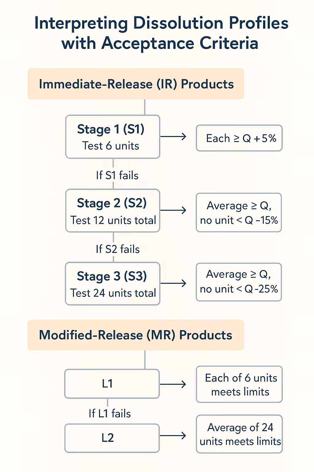
1. Immediate-Release (IR) Products
For IR tablets and capsules, the USP staged testing scheme is the global benchmark:
- Stage 1 (S1): Test 6 units. Each must be ≥ Q + 5%.
- Stage 2 (S2): If S1 fails, test 12 units total. The average must be ≥ Q, with no unit < Q − 15%.
- Stage 3 (S3): If S2 fails, test 24 units total. The average must be ≥ Q, with no unit < Q − 25%.
Action Point
Define your Q value (e.g., ≥ 80% dissolved in 30 min) based on compendial standards, clinical performance, or reference product data.
2. Modified-Release (MR) Products
MR formulations require multi-point specifications to capture release kinetics:
- Example: 20–30% at 1 h, 40–60% at 4 h, NLT 80% at 12 h.
- Evaluate against L1, L2, L3 criteria (similar logic to IR but applied at each time point).
Action Point
Ensure acceptance ranges are biologically relevant (IVIVC or PK data) and consistent with reference/innovator product performance.
3. Statistical Justification of Limits
- Acceptance criteria must not only be pharmacopeial but scientifically justified.
- Consider:
- Innovator/reference product profiles (for generics).
- Historical variability from manufacturing data.
- Clinical performance requirements.
Action Point
Document the scientific rationale for each acceptance criterion in your regulatory submission (CMC).
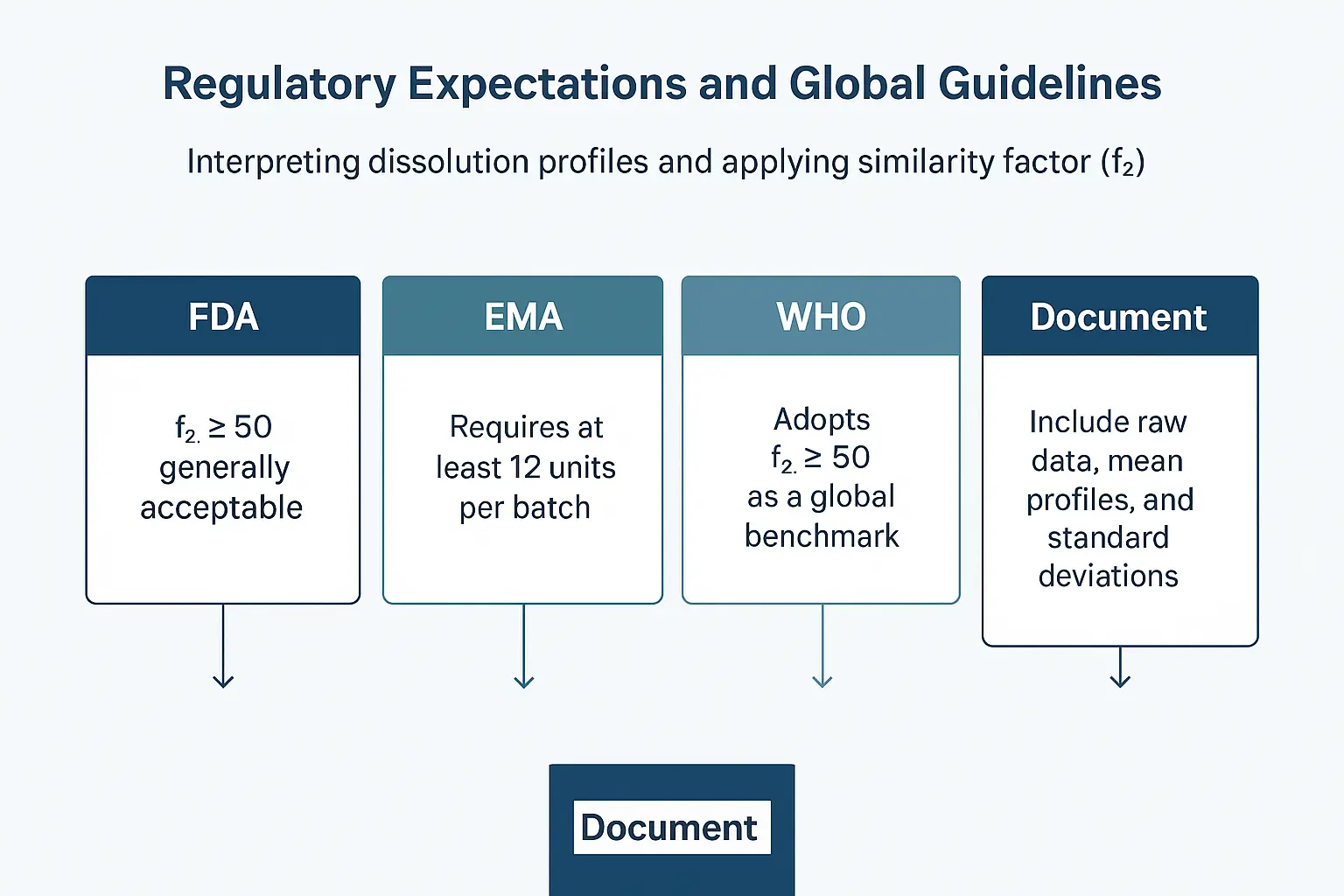
Step 10: Regulatory Expectations and Global Guidelines
Interpreting dissolution profiles and applying similarity factors (f₂) isn’t just a scientific exercise — it has direct regulatory implications. Regulatory agencies such as the U.S. Food and Drug Administration (FDA), European Medicines Agency (EMA), and World Health Organization (WHO) provide structured guidelines for how dissolution studies should be designed, analyzed, and reported.
🔹 Action Steps
Review FDA Guidance (SUPAC & Biowaiver Criteria)
- FDA’s Scale-Up and Post-Approval Changes (SUPAC) guidance specifies that f₂ ≥ 50 is generally acceptable to demonstrate similarity.
- For Biopharmaceutics Classification System (BCS) Class I drugs (high solubility, high permeability), dissolution similarity may allow biowaivers.
- Reference: FDA Guidance for Industry :Dissolution Testing of Immediate Release Solid Oral Dosage Forms
Consult EMA Guideline on Biowaivers
- EMA requires at least 12 units per batch and recommends use of f₂ where appropriate.
- Comparative dissolution should cover three pH conditions: 1.2, 4.5, and 6.8.
- 📖 Reference: EMA Guideline on the Investigation of Bioequivalence
Understand WHO Standards for Global Submissions
- WHO adopts f₂ ≥ 50 as a global benchmark for similarity.
- Emphasizes robustness of testing conditions and justification of media.
Document with Transparency
- Always include raw data, mean profiles, standard deviations, and the exact formula used for f₂.
- Provide justification for test conditions (apparatus, media, rpm) as part of your regulatory dossier.
Case Study & Practical Application
To bring everything together, let’s examine a real-world case study where dissolution profiles and the similarity factor (f₂) are applied to support product development and regulatory submission.
Case Study: Immediate-Release Paracetamol 500 mg Tablets
Scenario:
A generic manufacturer is developing Paracetamol 500 mg tablets and must demonstrate that their formulation is bioequivalent to the reference listed drug (RLD). Dissolution testing is performed at pH 1.2, 4.5, and 6.8 to simulate the GI tract conditions.
Step 1 — Collect Data
- Six units of both test and reference products are tested at each pH condition.
- Dissolution samples are collected at 5, 10, 15, 30, and 45 minutes.
Step 2 — Generate Profiles
- Dissolution curves are plotted for both formulations at each pH level.
- The profiles show >85% drug release by 30 minutes for both products.
Step 3 — Calculate Similarity Factor (f₂)
- At pH 1.2: f₂ = 65 → Profiles are similar.
- At pH 4.5: f₂ = 68 → Profiles are similar.
- At pH 6.8: f₂ = 74 → Profiles are similar.
Step 4 — Interpretation
- Since all f₂ values fall within 50–100, the profiles are statistically similar.
- This supports the claim that the test product will behave similarly to the reference in vivo.
Step 5 — Regulatory Context
- Both FDA and EMA guidelines accept f₂ ≥ 50 as evidence of similarity.
- Additional biowaiver justification is possible since paracetamol is a BCS Class I drug (high solubility, high permeability).
Actionable Takeaway
When preparing dissolution profiles for regulatory submission:
- Always test across multiple pH conditions.
- Use at least 12 units per profile for robust statistics.
- Confirm f₂ ≥ 50 across all physiological media.
- Justify with BCS classification and reference product performance.
- Document thoroughly in the CMC section with raw data, graphs, and statistical analysis.
Watch Those informative videos.